Excel:Formatting the elements of a graph
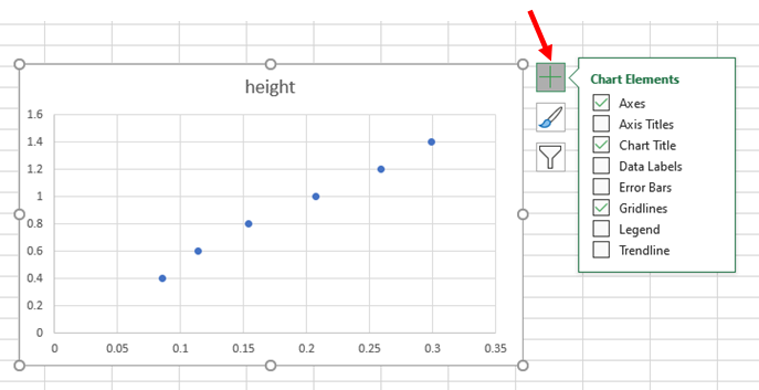
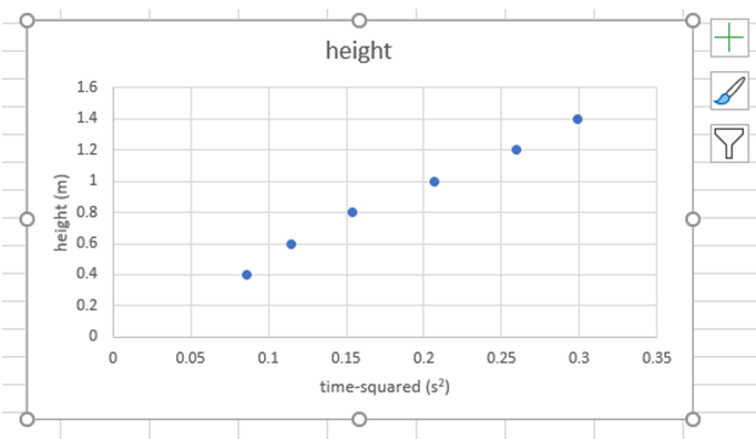
We have made a graph, now we will format the chart elements such as labeling the axes, changing the shape, size and color of the points. We can do all these things by clicking on the + sign on the right of the graph.1: If you click once on the + sign, you will see the following. If you don't see the plus sign, place the mouse over the graph and click once.
2: To put names for the axes, place the mouse pointer over 'Axis Title' and select it by a mouse click. You will see "Axis Title" text below the $x$ axis and before the $y$ axis.
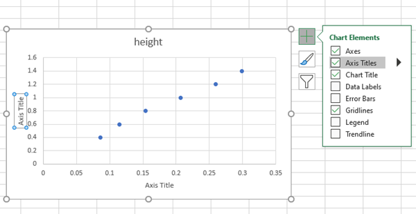
Now you can rename them and put whatever the name you want.
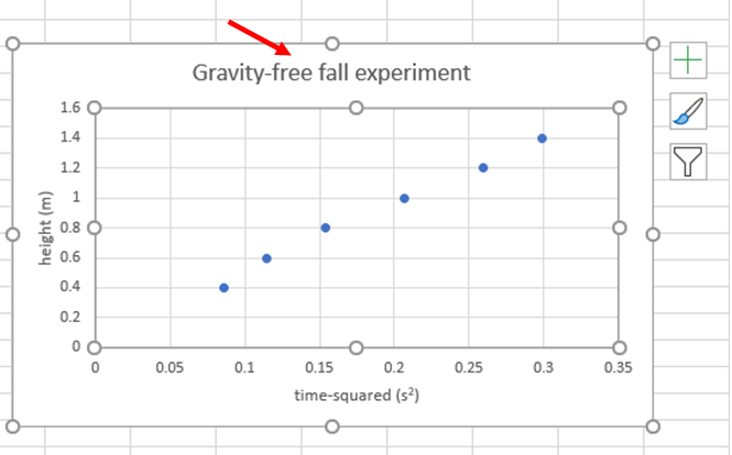
3: To rename the $x$ axis name, place the mouse pointer over "Axis Title" text and click once, and you will see the following.
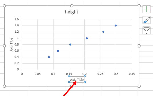
4: Click one more time so that you can delete the old text and enter the new desired text.
Do the same for the $y$ axis name. And, also to change the title of the graph.
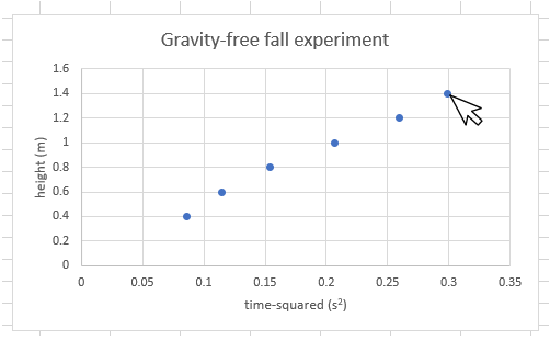
5: To change the color of the points' dots, place the mouse pointer on one of the dot and click once.
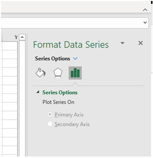
You will see the following on the right hand side of the excel window.
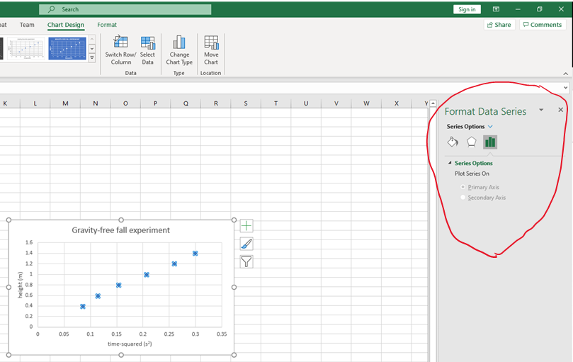
The expanded view of the circled area is as follows:
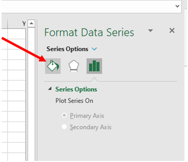
6: Place the mouse pointer on the icon (Fill & line) as shown.
7:Next, place the mouse pointer on the "marker"
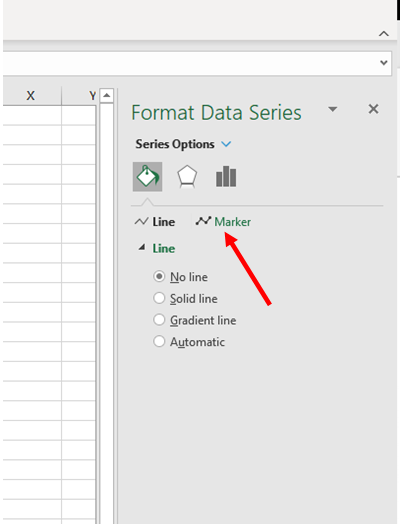
8: Click the mouse, you will see the following
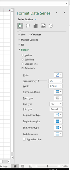
9: Place the mouse on the "Marker Options".
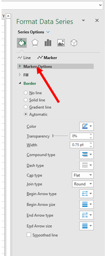
10: Click the mouse, you will see the following,
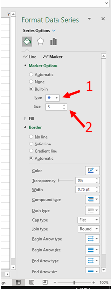
11: Use "Type" (1) and "Size" (2) to change the type and size of the points.
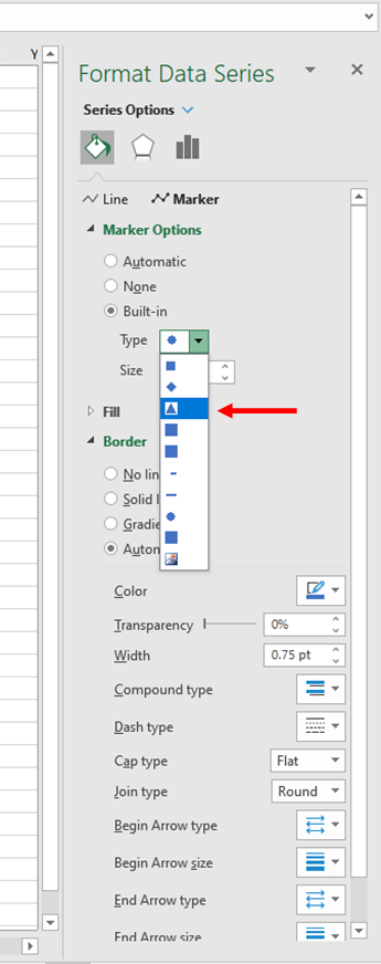
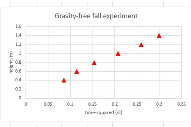
I changed the type to triangle and and also increase the size from 5 to 10 pts.
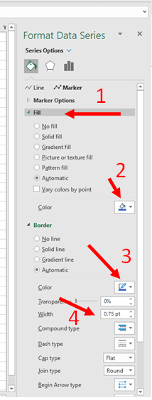
12: To change the color, move the mouse pointer to "Fill" (1) and click once to expand. To change the filling color, go to "Color" (2) and change that. To change the border color, go to "Color" (3) and change there. To change the thickness of the border go to "Width" (4) and change it.
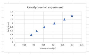
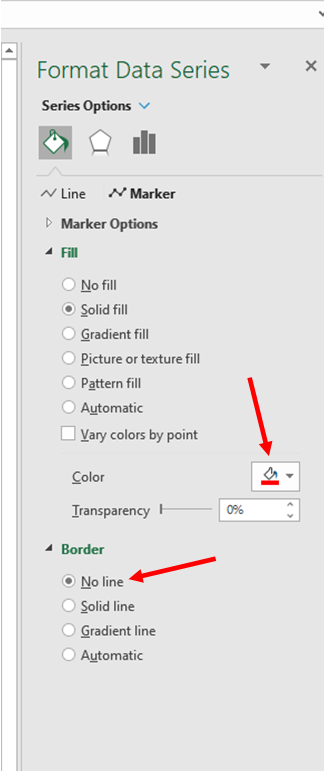
I chose red, and no border line.
The graph is now,