Excel: entering data
To learn excel, we will use the following data in the table from a "gravity and free fall" experiment.
In the experiment a ball was dropped at different heights and for each height, the time the ball took to hit the ground was measured. The purpose of this experiment is to find the acceleration due to gravity, $g$.
| S.no. | Drop height $h$ $(m)$ |
time $t$ $(s)$ |
Square of time $ t^2$ $(s^2)$ |
|---|---|---|---|
| 1 | 0.4 | 0.293 | |
| 2 | 0.6 | 0.338 | |
| 3 | 0.8 | 0.392 | |
| 4 | 1.0 | 0.455 | |
| 5 | 1.2 | 0.509 | |
| 6 | 1.4 | 0.547 |
The height, $h$ and the time, $t$ are related by the 1-D free fall equation:
$h=\dfrac{1}{2}gt^2$
So, if you draw a graph of $h$ vs $t^2$ with $t^2$ on the $x$ axis and $h$ on the $y$ axis, then you should get a straight line. The slope of the straight line is related to the $g$ by
Slope$=\dfrac{1}{2}g$
From this equation, you can find the $g$,
$g=2\cdot$slope
Since due to the experimental imperfections, you will not get a perfect straight line, if you draw $h$ vs $t^2$. So, you will find a straight line that is a best fit for all the experimental points and that line is called "trend line." Then you will find the slope of the trend line and will use that slope in the above equation to find $g$.
First we will enter the height and the time data in excel, then with the excel we will find the square of the time values.
Open excel and enter the data
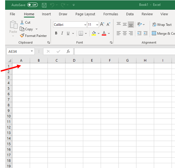
1: Open excel by clicking on the program icon or on the app.
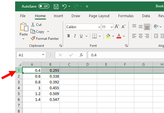
2: First we are going to enter the number, $0.4$, the first height value, in the cell pointed to by the red arrow in the figure below. The cell is the $A1$ cell as it is in column $A$ and in row $1$. Bring the mouse pointer ![]() on the A1 cell and double click.
on the A1 cell and double click.
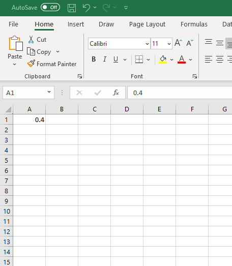
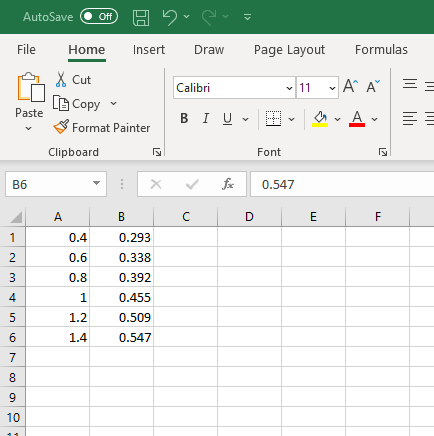
After double click, you are ready to enter the number on that cell with your keyboard. Type the number $0.4$.
3: Move the mouse pointer to the next cell, A2 in the same column, double click and enter 0.6. Repeat this to fill the other cells of the column up to row 6 with the other values of the height.
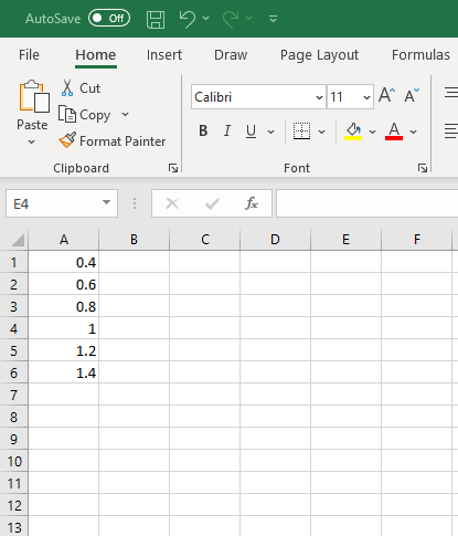
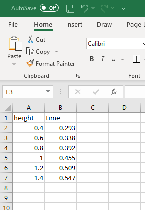
4: We have filled the first column, column A with the "height" values. Now fill the second (Column B) with the "time" values.
5: Now let us put a name for the columns: column A and column B so that we can easily identify them.
To put names, we need to insert a row above the current row 1. Move the mouse pointer over to the number "1", and click once to select that row.
Next right click the mouse and select "insert",
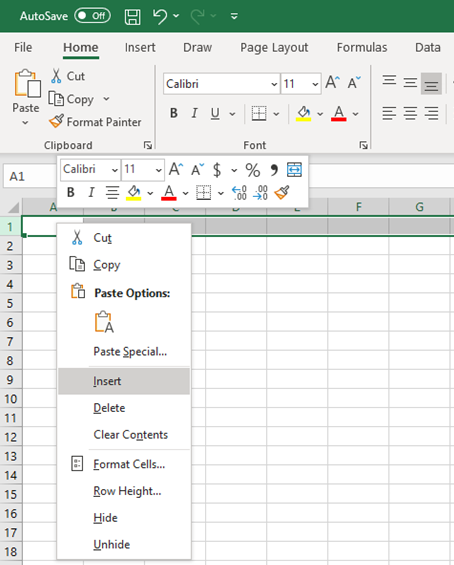
Once "click" insert, you will see a new blank row above the data.
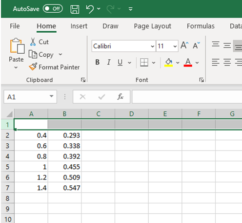
Now enter a name for each column. I have named "height" for the first column as it represents the height values, and the second column, "time" as it represents the time values.